Improve your R Markdown Skills

class: center, middle, inverse, title-slide

.title[
# Improve your R Markdown Skills
]
.author[
### Christophe Dervieux - Yihui Xie
]
.date[
### Raukr 2022 - 13/06/2022
]

---

# Who are we?

.subtitle[Short intro]

.center[

.profile[![:scale 20%, profile picture for Christophe Dervieux](https://avatars.githubusercontent.com/u/6791940?v=4)]

Christophe DERVIEUX &#8226; France

RStudio &#8226; Software Engineer &#8226; R Markdown Team

]
</br>
.pull-left[
.center[
.f2.color1[<svg aria-hidden="true" role="img" viewBox="0 0 496 512" style="height:1em;width:0.97em;vertical-align:-0.125em;margin-left:auto;margin-right:auto;font-size:inherit;fill:currentColor;overflow:visible;position:relative;"><path d="M165.9 397.4c0 2-2.3 3.6-5.2 3.6-3.3.3-5.6-1.3-5.6-3.6 0-2 2.3-3.6 5.2-3.6 3-.3 5.6 1.3 5.6 3.6zm-31.1-4.5c-.7 2 1.3 4.3 4.3 4.9 2.6 1 5.6 0 6.2-2s-1.3-4.3-4.3-5.2c-2.6-.7-5.5.3-6.2 2.3zm44.2-1.7c-2.9.7-4.9 2.6-4.6 4.9.3 2 2.9 3.3 5.9 2.6 2.9-.7 4.9-2.6 4.6-4.6-.3-1.9-3-3.2-5.9-2.9zM244.8 8C106.1 8 0 113.3 0 252c0 110.9 69.8 205.8 169.5 239.2 12.8 2.3 17.3-5.6 17.3-12.1 0-6.2-.3-40.4-.3-61.4 0 0-70 15-84.7-29.8 0 0-11.4-29.1-27.8-36.6 0 0-22.9-15.7 1.6-15.4 0 0 24.9 2 38.6 25.8 21.9 38.6 58.6 27.5 72.9 20.9 2.3-16 8.8-27.1 16-33.7-55.9-6.2-112.3-14.3-112.3-110.5 0-27.5 7.6-41.3 23.6-58.9-2.6-6.5-11.1-33.3 2.6-67.9 20.9-6.5 69 27 69 27 20-5.6 41.5-8.5 62.8-8.5s42.8 2.9 62.8 8.5c0 0 48.1-33.6 69-27 13.7 34.7 5.2 61.4 2.6 67.9 16 17.7 25.8 31.5 25.8 58.9 0 96.5-58.9 104.2-114.8 110.5 9.2 7.9 17 22.9 17 46.4 0 33.7-.3 75.4-.3 83.6 0 6.5 4.6 14.4 17.3 12.1C428.2 457.8 496 362.9 496 252 496 113.3 383.5 8 244.8 8zM97.2 352.9c-1.3 1-1 3.3.7 5.2 1.6 1.6 3.9 2.3 5.2 1 1.3-1 1-3.3-.7-5.2-1.6-1.6-3.9-2.3-5.2-1zm-10.8-8.1c-.7 1.3.3 2.9 2.3 3.9 1.6 1 3.6.7 4.3-.7.7-1.3-.3-2.9-2.3-3.9-2-.6-3.6-.3-4.3.7zm32.4 35.6c-1.6 1.3-1 4.3 1.3 6.2 2.3 2.3 5.2 2.6 6.5 1 1.3-1.3.7-4.3-1.3-6.2-2.2-2.3-5.2-2.6-6.5-1zm-11.4-14.7c-1.6 1-1.6 3.6 0 5.9 1.6 2.3 4.3 3.3 5.6 2.3 1.6-1.3 1.6-3.9 0-6.2-1.4-2.3-4-3.3-5.6-2z"/></svg>]</br>
[@cderv](https://github.com/cderv)
]
]

.pull-right[
.center[
.f2.color1[<svg aria-hidden="true" role="img" viewBox="0 0 512 512" style="height:1em;width:1em;vertical-align:-0.125em;margin-left:auto;margin-right:auto;font-size:inherit;fill:currentColor;overflow:visible;position:relative;"><path d="M459.37 151.716c.325 4.548.325 9.097.325 13.645 0 138.72-105.583 298.558-298.558 298.558-59.452 0-114.68-17.219-161.137-47.106 8.447.974 16.568 1.299 25.34 1.299 49.055 0 94.213-16.568 130.274-44.832-46.132-.975-84.792-31.188-98.112-72.772 6.498.974 12.995 1.624 19.818 1.624 9.421 0 18.843-1.3 27.614-3.573-48.081-9.747-84.143-51.98-84.143-102.985v-1.299c13.969 7.797 30.214 12.67 47.431 13.319-28.264-18.843-46.781-51.005-46.781-87.391 0-19.492 5.197-37.36 14.294-52.954 51.655 63.675 129.3 105.258 216.365 109.807-1.624-7.797-2.599-15.918-2.599-24.04 0-57.828 46.782-104.934 104.934-104.934 30.213 0 57.502 12.67 76.67 33.137 23.715-4.548 46.456-13.32 66.599-25.34-7.798 24.366-24.366 44.833-46.132 57.827 21.117-2.273 41.584-8.122 60.426-16.243-14.292 20.791-32.161 39.308-52.628 54.253z"/></svg>]</br>
[@chrisderv](https://twitter.com/chrisderv)
]
]

???

---

# Who are we?

.subtitle[Short intro]

.center[

.profile[![:scale 20%, profile picture for Yihui Xie](https://avatars.githubusercontent.com/u/163582?v=4)]

Yihui XIE &#8226; USA

RStudio &#8226; Software Engineer &#8226; R Markdown Team

---
# What are we talking today ?

.pull-left.center[
![:scale 75%, rmarkdown package logo](https://pkgs.rstudio.com/rmarkdown/reference/figures/logo.png)
.f5[https://pkgs.rstudio.com/rmarkdown/]
]
.pull-right.center[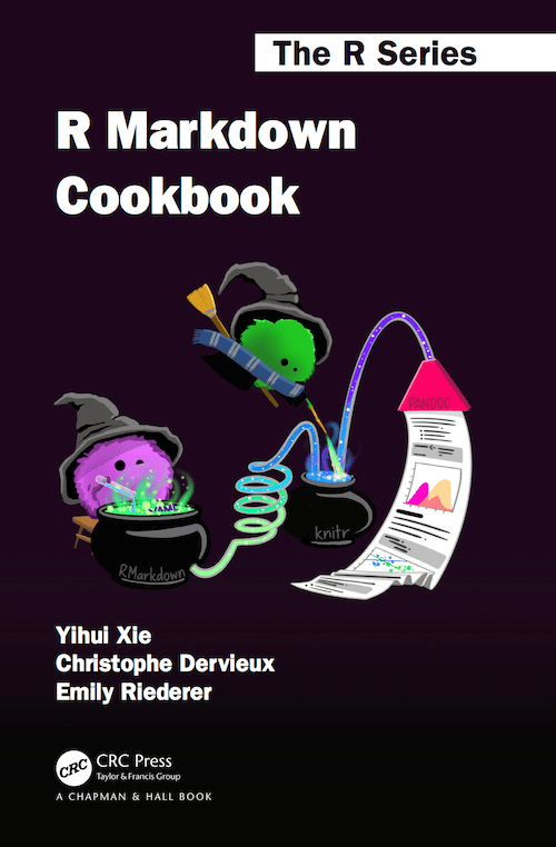
![:scale 55%, R Markdown Cookbook book cover](https://bookdown.org/yihui/rmarkdown-cookbook/images/cover.png)
.f5[https://bookdown.org/yihui/rmarkdown-cookbook/]
]
???

Everyone should know rmarkdown among R users. Its principle has not changed since a long time 
(md + R = Rmd -> output format) quite easy to start (write text, add code chunk, compile) but it can be harder to learn new skill to be more efficient and get full power.

That is where known recipes can help master more advanced skills. R Markdown Cookbook was thought as a non linear documentation.

Also new logo and new pkgdown website

---
layout: true

# What happens when it renders ?

---

.center[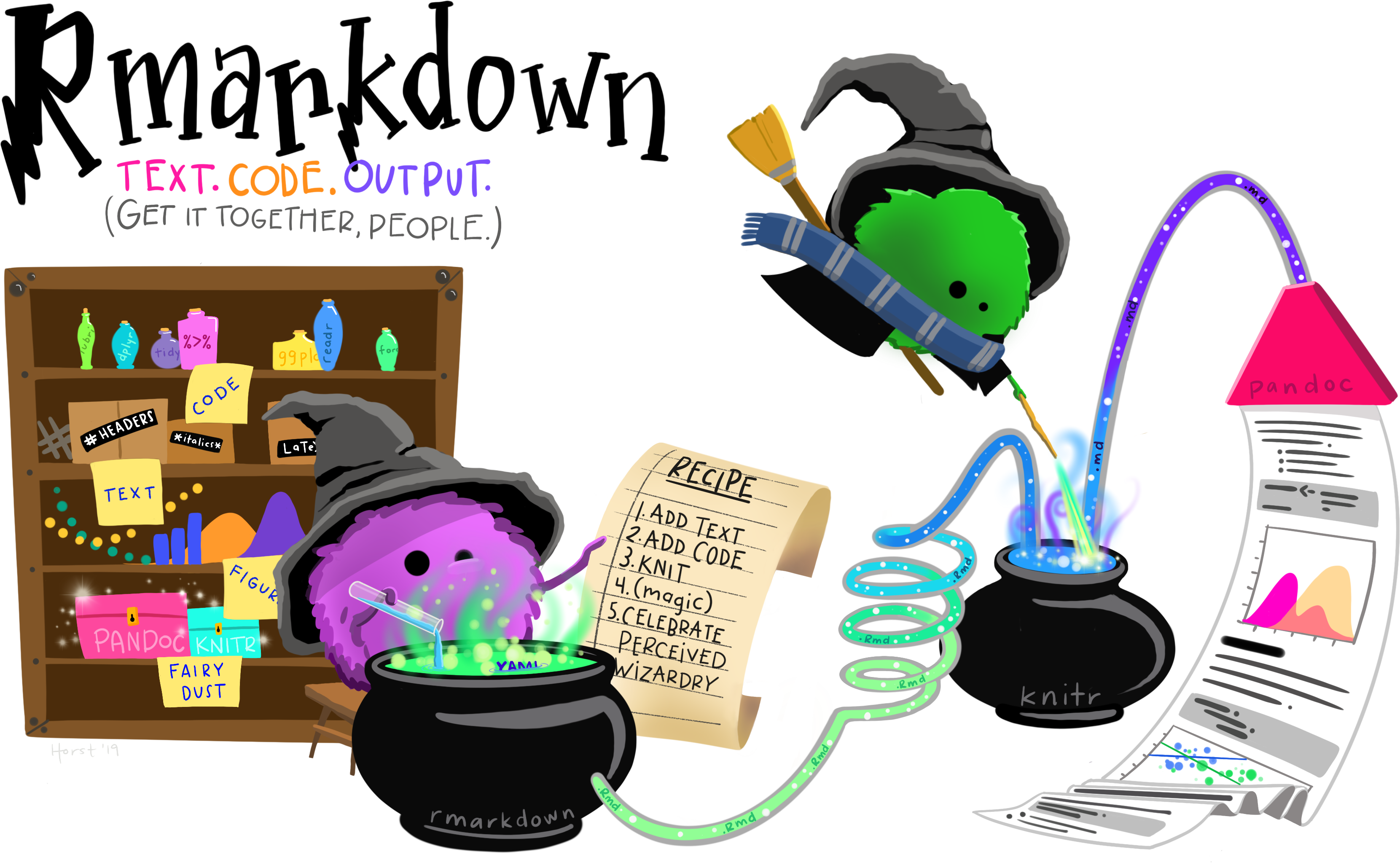![:scale 75%, R Markdown wizard illustration by Alison Horst](rmarkdown_wizards.png)]
.source-fig.center[Source: https://github.com/allisonhorst/stats-illustrations]

???

We often see these rmarkdown little wizard mixing Text & Code to produce document. Aim is to look deeper into this today. This is not so magic. It is juts percieved magic and there are tools to know about under the hood to be able to customize behavior further.

---

.center[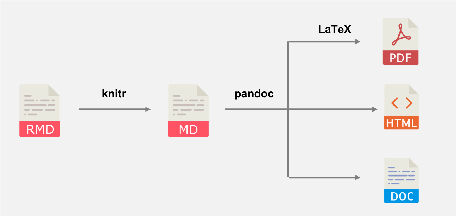![:scale 80%, Diagram showing the different step of rendering, using knitr first from Rmd to md, then Pandoc from md to output format like HTML, DOC and PDF (using LaTeX)](https://bookdown.org/yihui/rmarkdown-cookbook/images/workflow.png)]
.source-fig.center[
source: [R Markdown Cookbook](https://bookdown.org/yihui/rmarkdown-cookbook)
]

.box.f3[`knitr::knit()` + Pandoc (+ LaTeX for PDF) = `rmarkdown::render()`]

???

rmarkdown will run Pandoc & knitr for you.

LaTeX only needed with PDF. tinytex will run it for you.

This is important to know all this because it helps know where to look and what could be tweak. one has to understand what to tweak to make something works as expected.

---
layout: false

# About the tools

.subtitle[We got you covered!]

* **rmarkdown** 📦 will install **knitr** and **tinytex** for you
* _Pandoc_ is an external binary tool, .color1.underline[included] inside RStudio IDE. 
* _TinyTeX_ is the only thing to install if you want PDF output. (`tinytex::install_tinytex()`)

.pull-left[

In case you need it:
(.small[but you probably won't!])

* [Use another Pandoc version](https://bookdown.org/yihui/rmarkdown-cookbook/install-pandoc.html) (should never be necessary!)
* [Install missing LaTeX package](https://bookdown.org/yihui/rmarkdown-cookbook/install-latex-pkgs.html) (should not be necessary as **tinytex** will do it for you at render)
]

.pull-right[
![](https://bookdown.org/yihui/rmarkdown-cookbook/images/workflow.png)

.right[.small[source: [R Markdown Cookbook](https://bookdown.org/yihui/rmarkdown-cookbook)]]
]

???

Best to use TinyTeX as it is tested agains rmarkdown.

Everything should work as expected otherwise. No special tool needed unless for advanced usage.

Missing CTAN packages are installed by tinytex the R package.

---
# Let's dive now !

.center[![:scale 60%, Illustration by Allison Horst about R Markdown being a band with Text playing the batterie, outputs singing and code plyaing the guitar!](https://github.com/allisonhorst/stats-illustrations/raw/master/rstats-artwork/rmarkdown_rockstar.png)]
.source-fig.center[Source: https://github.com/allisonhorst/stats-illustrations]

???

Not sure the aim is to be a rockstar but for sure it is to make those three little guy playing together smoothly

---

# How to boost content creation ?

.center[![:scale 50%, Gif sayins Content is king with an illustration of a king at his desk in front of a computer with a crown dropping on his head. ](https://media.giphy.com/media/ymTxohR7QWdAOBuYtC/giphy.gif)]

???

First thing to focus one: Boost the content of the R Markdown.
---

# Writing long chunk options

.ribbon[
New in **knitr**
]

.subtitle[About the chunk header syntax `#|`]

Using R syntax (`tag = value`, comma-separated, arbitrary line-wrapping)

````markdown
```{r}
#| echo = FALSE, fig.width = 10,
#| fig.cap = "This is a long caption."

plot(cars)
```
````

Using YAML syntax (`tag: value`; one chunk option per line)

````markdown
```{r}
#| echo: FALSE
#| fig.width: 10
#| fig.cap: "This is a long caption."

plot(cars)
```
````

---

# Read external scripts into a chunk

.ribbon[
New in **knitr**
]

.subtitle[About the `file` chunk option]

.panelset[

.panel[.panel-name[in my_script.R]

```r
add <- function(x, y) {
  x + y
}
```
]

.panel[.panel-name[in your Rmd]

````markdown
```{r, file = 'my_script.R'}
```
````

]

.panel[.panel-name[equivalent to]

````markdown
```{r}
add <- function(x, y) {
  x + y
}
```
````

]

.panel[.panel-name[previous way]

.small[Which is still working]

````markdown
```{r, code = xfun::read_utf8('my_script.R')}
```
````
]

]

* This will fill the content of the chunk

* Can be used with any engine (R, Python, C++, ...)

* Can be used with multiple scripts (e.g `file = c("foo.R", "bar.R")`)

???

From Bookdown : https://bookdown.org/yihui/rmarkdown-cookbook/option-code.html

Useful for bigger project, or when script already exists.

---

# Construct chunk content from a variable

.subtitle[About the `code` chunk option]

Example: Installation instruction for packages.

````markdown
```{r, include = FALSE}
pkgs <- c("glue", "fs")
install_code <- sprintf('install.packages("%s")', pkgs)
```
*```{r, eval = FALSE, code = install_code}
```
````

renders without evaluating to

```r
install.packages("glue")
install.packages("fs")
```

???

This is just an example and this can be done with any chunk option. It is quite powerful !

---

# Read code chunks from a script

.subtitle[About `knitr::read_chunk()`]

.panelset[

.panel[.panel-name[my_script.R]

Use a special comment syntax to label code content.

```r
## ---- chunk-label
```
Ex in `my_chunks.R`

````r
## ---- my-chunk-a --------
1 + 1

## ---- my-chunk-b --------
plot(cars)
```` 
]

.panel[.panel-name[report.Rmd]

````markdown
Read an external script to load chunks:

```{r, include=FALSE, cache=FALSE}
*knitr::read_chunk('my_script.R')
```

Now the code can be used chunk by chunk, e.g.,

```{r, my-chunk-a, echo=FALSE}
```

```{r, my-chunk-b, fig.height=4}
```
````

]

???

Useful for:

* sharing common part of code in a script
* Store all R code in one R file
* For bigger project often, or when script already exists.

https://bookdown.org/yihui/rmarkdown-cookbook/read-chunk.html

---

# Use Rmd child document

.subtitle[About `child` chunk option]

Reuse the same content across several Rmd documents:

````markdown
```{r child = "_common.Rmd"}
```
````
.small[Also used often with `include = FALSE` to load common setup content as setup chunk in several documents.]

Conditionally include some content:

````markdown
Change `BOSS_MODE` to `TRUE` if this report is to be read by the boss:

```{r, include=FALSE}
# variable impacting the rendering, which could be a parameter of a report
*BOSS_MODE <- FALSE
```

Conditionally include the appendix:

*```{r, child = if (!BOSS_MODE) 'appendix.Rmd'}
```
````

???

This respect chunk option so could be useful for conditionnally eval or not a part of a document.

Also useful to organize project in smaller pieces.

https://bookdown.org/yihui/rmarkdown-cookbook/child-document.html

---

# Dynamically create content

.subtitle[About `knitr::knit_child()`</br>(and `result = 'asis'`)]

.panelset[
.panel[
.panel-name[`template.Rmd`]

````markdown
## Regression on `r x`

```{r}
lm(mpg ~ ., data = mtcars[, c("mpg", x)])
```
````

* We want to apply one linear regression between `mpg` and each of other variables of `mtcars` 
```r
# select other variables than 'mpg'
x_vars <- setdiff(names(mtcars), 'mpg')
```
* We want the result to be included in .color2[its in own chapter].
]
.panel[.panel-name[`main.Rmd`]

````markdown
*```{r, echo=FALSE, results='asis'}
# select other variables than 'mpg'
x_vars <- setdiff(names(mtcars), 'mpg')
# knit the template for each
res <- lapply(x_vars, function(x) {
*   knitr::knit_child('template.Rmd', 
    envir = environment(), quiet = TRUE
  )
})
# cat() the knitted output to be included 'asis' 
*cat(unlist(res), sep = '\n')
```
````

Can be combined with [`knitr::knit_expand()`](https://bookdown.org/yihui/rmarkdown-cookbook/knit-expand.html)

]
.panel[.panel-name[without external file]

````markdown
```{r, echo=FALSE}
x_vars <- setdiff(names(mtcars), 'mpg')
res <- lapply(x_vars, function(x) {
*  knitr::knit_child(text = c(
    '## Regression on "`r x`"',
    '',
    '```{r}',
    'lm(mpg ~ ., data = mtcars[, c("mpg", x)])',
    '```',
    ''
  ), envir = environment(), quiet = TRUE)
})
*res <- paste(res, collapse = "\n") # create one string with content
```

*`r res`

````
]
]

???

Quite like child document but a bit different. Can be useful sometimes for programatically create markdown content.

https://bookdown.org/yihui/rmarkdown-cookbook/child-document.html

---

# Reuse a chunk

.subtitle[About chunk `label`]

````markdown
Here is a code chunk that is not evaluated:

*```{r, chunk-one, eval = FALSE}
1 + 1
2 + 2
```

Now we actually evaluate it:

*```{r, chunk-one, eval = TRUE}
```
````

First chunk will be used twice - different options are allowed.

???

Reuse a figure, Show code in another place that the initial result, show figure in another place than where the plot has been evaluated. Recompute the same content.

https://bookdown.org/yihui/rmarkdown-cookbook/reuse-chunks.html

---

# Use labels to reference chunks

.subtitle[About chunk `ref.label`]

.panelset[

.panel[.panel-name[Rmd code]

````markdown

```{r chunk-b, echo = FALSE}
# this is the chunk b
1 + 1
```

```{r chunk-c, echo = FALSE}
# this is the chunk c
2 + 2
```
*```{r chunk-a, ref.label = c('chunk-c', 'chunk-b'), eval = FALSE}
```

````
]

.panel[.panel-name[`chunk-a` equivalent to]

````markdown
```{r chunk-a, eval = FALSE}
# this is the chunk c
2 + 2
# this is the chunk b
1 + 1
```
````

]

.panel[.panel-name[knitted md output]

````markdown
```
## [1] 2
```

```
## [1] 4
```

```r
# this is the chunk c
2 + 2
# this is the chunk b
1 + 1
```
````

]

???

Yes chunk content can be combined. Could be useful to show code in appendix at the end of the document for example.

https://bookdown.org/yihui/rmarkdown-cookbook/reuse-chunks.html

---

# Include content verbatim (1)

.ribbon[
New in **knitr**
]

.subtitle[About `verbatim` engine]

.panelset[

.panel[.panel-name[in your Rmd]

````markdown

Let's show an example of Rmd file content:

*````{verbatim, lang = "markdown"}
We can output arbitrary content **verbatim**.

```{r}
1 + 1
```

The content can contain inline code like
`r pi * 5^2`, too.
*````
````

]

.panel[.panel-name[after knit in md file]

````markdown
Let's show an example of Rmd file content:

*````markdown
We can output arbitrary content **verbatim**.

```{r}
1 + 1
```

The content can contain inline code like
`r pi * 5^2`, too.
*````
````

]

See also about `knitr::inline_expr()` to [Show a verbatim inline expression](https://bookdown.org/yihui/rmarkdown-cookbook/verbatim-code-chunks.html#show-a-verbatim-inline-expression)

---

# Include content verbatim (2)

.ribbon[
New in **knitr**
]

.subtitle[About `embed` engine]

.panelset[

.panel[.panel-name[`macros.js`]

Here is the `macros.js` content used for _remark.js_ with this **xaringan** presentation

```js
remark.macros.scale = function(w, alt="") {
  var url = this;
  return '<img src="' + url + '" style="width: ' + w + ';" alt="' + alt + '" />';
};
remark.macros.scaleh = function(h, alt="") {
  var url = this;
  return '<img src="' + url + '" style="height: ' + h + ';" alt="' + alt + '" />';
};
```

]

.panel[.panel-name[inside Rmd file]

````markdown
Here is the `macros.js` content used for _remark.js_ with this **xaringan** presentation

*```{embed, file = "macros.js"}
```
````

]

.panel[.panel-name[after knit in md file]

````markdown
Here is the `macros.js` content used for _remark.js_ with this **xaringan** presentation

*```js
remark.macros.scale = function(w, alt="") {
  var url = this;
  return '<img src="' + url + '" style="width: ' + w + ';" alt="' + alt + '" />';
};
remark.macros.scaleh = function(h, alt="") {
  var url = this;
  return '<img src="' + url + '" style="height: ' + h + ';" alt="' + alt + '" />';
};
```
````

]

* Language used for code blocks is derived from file extension
* It can be customized using the `lang` option
* Equivalent to using `verbatim` engine with `lang` and `code` chunk options... but simpler to use !

???

https://bookdown.org/yihui/rmarkdown-cookbook/verbatim-code-chunks.html#verbatim-code-chunks

---

# Using any command-line tools in a chunk (1)

.ribbon[
New in **knitr**
]

.subtitle[About the `exec` engine]

The `exec` engine allows to execute an arbitrary command on the code chunk
content, optionally with arguments.

</br>

.panelset[

.panel[.panel-name[In your Rmd file]

````markdown
```{exec, command='Rscript', engine.opts = list(args1 = "--vanilla")}
1 + 1
```
````

]

.panel[.panel-name[after knit in md file]
````markdown

```r
1 + 1
```

```
## [1] 2
```
````

]

For details about this new engine, see [`124-exec-engine.Rmd`](https://github.com/yihui/knitr-examples/blob/master/124-exec-engine.Rmd) in [knitr-examples repo](https://github.com/yihui/knitr-examples).

???

The `exec` engine allows to execute an arbitrary command on the code chunk
content, optionally with arguments. If any, they are passed to `engine.opts` and
they could be one of the following:

---

# Using any command-line tools in a chunk (2)

.ribbon[
New in **knitr**
]

.subtitle[More complexe example using `awk`]

.panelset[

.panel[.panel-name[`marks.txt`]

```txt
1) Amit Physics 80
2) Rahul Maths 90
3) Shyam Biology 87
4) Kedar Maths 85
5) Hari History 89
```

Let's try process this file with `awk` from within our R Markdown document

]

.panel[.panel-name[in Rmd file]

````markdown
Let's count how many line contains `Maths`

```{exec, command = "awk", engine.opts = list(args1 = "-f", args2 = "marks.txt")}
/Maths/{++cnt} END {print "Count = ", cnt}
```
````

* `args1 = "-f"` needed to execute the content of the chunk as a `awk` program
* `args2` is used to pass the text file to process with the program

]

.panel[.panel-name[after knit in md file]

````markdown

Let's count how many line contains `Maths`

```awk
/Maths/{++cnt} END {print "Count = ", cnt}
```

```
## Count =  2
```
````

See [`124-exec-engine.Rmd`](https://github.com/yihui/knitr-examples/blob/master/124-exec-engine.Rmd) in [knitr-examples repo](https://github.com/yihui/knitr-examples) for the different options.

]

???

Using some command line tools may require tweaking the `exec` engine arguments

---

# What about styling outputs ?

.center[![:scale 65%, Gif of a man in a suits putting a a pink hat with included sunglasses. Text on the gif says 'You don't like my style', then 'Deal with it'](https://media.giphy.com/media/14o3gppq0mt2Lu/giphy.gif)]

???

Let's talk about styling content now.

---

# Use CSS from inside a Rmd file

.subtitle[About the `css` engine]

````markdown
```{css, echo = FALSE}
/* add a blue border */
div.mybox {
  border-color: blue;
  border-style: solid;
  padding: 0.5em;
}

/* Set to blue bold text inside the box */
div.mybox strong {
  color: blue;
}
```
````

Applied directly in the Rmd document without an external css file

Going further: See the [`js` engine](https://bookdown.org/yihui/rmarkdown-cookbook/details-tag.html) to apply JS code the same way

???

Useful for prototyping, for quick iteration, for single file example
echo = false is important if you don't want to show CSS source chunk in output

---
layout: true
# Use SASS the same way

.subtitle[About the `sass`/`scss` engine]

---

### What is SASS ?

Sass (https://sass-lang.com) is a CSS extension language that allows you to create CSS rules in much more flexible ways than you would do with plain CSS.
</br>
</br>
.center[![:scale 25%](https://sass-lang.com/assets/img/logos/logo-b6e1ef6e.svg)]

It allows for variables, tweaking functions (called _mixins_), operations (like `/`), better CSS rule organisation (nesting, extensions, ...) and more.

???

External tool used by web developers. Very powerful and this is a skill to learn when doing a lot of HTML. It can do a lot !

But no need to use it directly. Still need to learn the feature and syntax.

---
.panelset[

.panel[.panel-name[previous css]

````markdown
```{css, echo = FALSE}
div.mybox {
* border-color: blue;
  border-style: solid;
  padding: 0.5em;
}

div.mybox strong {
* color: blue;
}
```
````

]

.panel[.panel-name[scss]
````markdown
```{scss, echo = FALSE}
*$color1: blue;

div {
  &.mybox {
*   border-color: $color1;
    border-style: solid;
    padding: 0.5em;

strong {
*     color: $color1;
    }
  }
}
```
````

]
.panel[.panel-name[sass]
````markdown
```{sass, echo = FALSE}
$color1: blue

div
  &.mybox
    border-color: $color1
    border-style: solid
    padding: 0.5em
  
    strong
      color: $color1
```
````
In both example, we are using special _SASS_ feature like [Nesting](https://sass-lang.com/documentation/style-rules/declarations#nesting) and [Parent Selector](https://sass-lang.com/documentation/style-rules/parent-selector).

]
]

???

The CSS is the one that would be render when using sass on the .scss or .sass file.

No preference on the syntax - it is a personnal choice (and depending on environment.)

---
layout: true
# Use SASS the same way

.subtitle[Powered by the new **sass** R 📦]

---

.center[

![:scale 25%](https://rstudio.github.io/sass/reference/figures/logo.svg)

https://rstudio.github.io/sass/

</br>
.box[Support is now built-in **rmarkdown**]

]

???

Quite new. Allow to use SASS from R. Wrapper around a C library.

Supported in rmarkdown now.

---

.panelset[

.panel[.panel-name[style.sass]

```sass
$color1: blue

div
  &.mybox
    border-color: $color1
    border-style: solid
    padding: 0.5em
  
    strong
      color: $color1
```

]

.panel[.panel-name[rendered CSS]

```r
# Rendering SASS file from R
sass::sass(sass::sass_file("style.sass"))
```

```{.css}
div.mybox {
  border-color: blue;
  border-style: solid;
  padding: 0.5em;
}

div.mybox strong {
  color: blue;
}
```

]

???

Small intro. Best is to look at the pkgdown website.

---

External `.sass` / `.scss` file can also be passed in the `css` argument of `html_document()`

</br>

````yaml
output:
  html_document:
    css: custom-style.scss
````

The file will be processed internally by `sass::sass_file()` and produce a `.css` automatically.

???

You can do much more with SASS. It pushes the limit of customization of a document.

How to use it ? Why this CSS example ?

---
layout: true

# Use custom blocks to style

.subtitle[Powered by Pandoc's fenced divs syntax]

---

```markdown
::: mybox
Special **important** content
:::
```

.mybox-demo strong {
  color: blue;
}
</style>

With the previous style applied, it will result in this box in the document
</br></br>
.mybox-demo[
Special **important** content
]
</br></br>

```html
<div class="mybox">
<p>Special <strong>important</strong> content</p>
</div>
```

???

Pandoc feature. R Markdown knows and extend it. 
Quite simple to write but quite powerful.

Supported by Visual editor.

---

Attributes and id can be added too, e.g

```markdown
::: {.mybox #box1 style="text-align: center;"}
Special **important** content
:::
```

The above add inline style to the div
</br></br>
.center.mybox-demo[
Special **important** content
]
</br></br>

```html
<div id="box1" class="mybox" style="text-align: center;">
<p>Special <strong>important</strong> content</p>
</div>
```

???

Allow to style mainly.

---
layout: true

# Aiming multi formats

.subtitle[About **rmarkdown** custom blocks for PDF support]

---

.panelset[

.panel[.panel-name[Support of latex]

```markdown
::: {.mybox latex=true}
Special **important** content
:::
```

]
.panel[.panel-name[will output in LaTeX]

```latex
\begin{mybox}
Special \textbf{important} content

\end{mybox}
```
]
]

Specially supported by R Markdown and not Pandoc.

.box[Create a LaTeX environment as easily as you can create a HTML div.]

???

Extend the Pandoc feature for LaTeX environment. Not done by default in Pandoc. 
Special feature of rmarkdown.

---

This requires a LaTeX preamble for this custom environment to render to PDF, e.g using `tcolorbox` CTAN package.

```latex
\usepackage{tcolorbox}
\newtcolorbox{mybox}{
  colframe=blue,
  halign=center,
  boxsep=5pt,
  arc=4pt}
```

To pass to the output format, e.g
```yaml
output: 
  pdf_document:
    includes:
      in_header: preamble.tex
```

???

Could also be added in a file directly obviously.

---

Using the `cat` engine can help you write the preamble from within the Rmd file

````markdown
```{cat, engine.opts = list(file = 'preamble.tex')}
\usepackage{tcolorbox}
\newtcolorbox{mybox}{
  colframe=blue,
  halign=center,
  boxsep=5pt,
  arc=4pt}
```
````

This will result in the PDF as this box

???

Just for showing cat engine usage here;

And try texPreview in source file

---
layout: false
class: middle

.center[

![:scale 55%, Gif with an image from The Fresh Prince of Bel-Air wearing a pink hat and in a position of thinking with right hand of its chin. Text has been added and says 'But what about the blue bold text ?'](but-why-not-blue2.gif)

LaTeX customization is a topic for another time ! 🙄

]

---
layout: false

# What we've learn so far ?

.subtitle[Let's sum up!]

## Be more powerfull with **knitr**

* .color2[**Include content verbatim**] from text or files
* .color2[**Import code chunk content**] from a script or from a variable
* .color2[**Use Rmd child document**] to share content in several places
* .color2[**Reuse some chunks**] several times
* .color2[**Use any CLI tools**] on the code chunk content

## Customize output style

* .color2[**Customize HTML output**] using CSS and SASS code
* .color2[**Create and style custom blocks**] for HTML and PDF allowing better customization

---

# How to go further ?

.subtitle[and boost even more your skills !]

.pull-left.center[

## Look at examples

Xaringan Source of this presentation in </br> .f2.color1[<svg aria-hidden="true" role="img" viewBox="0 0 496 512" style="height:1em;width:0.97em;vertical-align:-0.125em;margin-left:auto;margin-right:auto;font-size:inherit;fill:currentColor;overflow:visible;position:relative;"><path d="M165.9 397.4c0 2-2.3 3.6-5.2 3.6-3.3.3-5.6-1.3-5.6-3.6 0-2 2.3-3.6 5.2-3.6 3-.3 5.6 1.3 5.6 3.6zm-31.1-4.5c-.7 2 1.3 4.3 4.3 4.9 2.6 1 5.6 0 6.2-2s-1.3-4.3-4.3-5.2c-2.6-.7-5.5.3-6.2 2.3zm44.2-1.7c-2.9.7-4.9 2.6-4.6 4.9.3 2 2.9 3.3 5.9 2.6 2.9-.7 4.9-2.6 4.6-4.6-.3-1.9-3-3.2-5.9-2.9zM244.8 8C106.1 8 0 113.3 0 252c0 110.9 69.8 205.8 169.5 239.2 12.8 2.3 17.3-5.6 17.3-12.1 0-6.2-.3-40.4-.3-61.4 0 0-70 15-84.7-29.8 0 0-11.4-29.1-27.8-36.6 0 0-22.9-15.7 1.6-15.4 0 0 24.9 2 38.6 25.8 21.9 38.6 58.6 27.5 72.9 20.9 2.3-16 8.8-27.1 16-33.7-55.9-6.2-112.3-14.3-112.3-110.5 0-27.5 7.6-41.3 23.6-58.9-2.6-6.5-11.1-33.3 2.6-67.9 20.9-6.5 69 27 69 27 20-5.6 41.5-8.5 62.8-8.5s42.8 2.9 62.8 8.5c0 0 48.1-33.6 69-27 13.7 34.7 5.2 61.4 2.6 67.9 16 17.7 25.8 31.5 25.8 58.9 0 96.5-58.9 104.2-114.8 110.5 9.2 7.9 17 22.9 17 46.4 0 33.7-.3 75.4-.3 83.6 0 6.5 4.6 14.4 17.3 12.1C428.2 457.8 496 362.9 496 252 496 113.3 383.5 8 244.8 8zM97.2 352.9c-1.3 1-1 3.3.7 5.2 1.6 1.6 3.9 2.3 5.2 1 1.3-1 1-3.3-.7-5.2-1.6-1.6-3.9-2.3-5.2-1zm-10.8-8.1c-.7 1.3.3 2.9 2.3 3.9 1.6 1 3.6.7 4.3-.7.7-1.3-.3-2.9-2.3-3.9-2-.6-3.6-.3-4.3.7zm32.4 35.6c-1.6 1.3-1 4.3 1.3 6.2 2.3 2.3 5.2 2.6 6.5 1 1.3-1.3.7-4.3-1.3-6.2-2.2-2.3-5.2-2.6-6.5-1zm-11.4-14.7c-1.6 1-1.6 3.6 0 5.9 1.6 2.3 4.3 3.3 5.6 2.3 1.6-1.3 1.6-3.9 0-6.2-1.4-2.3-4-3.3-5.6-2z"/></svg>] [cderv/raukr-2022-rmd-skills](https://github.com/cderv/raukr-2022-rmd-skills)
</br></br></br>

]

.pull-right.center[

## More in the book

![:scale 40%](https://bookdown.org/yihui/rmarkdown-cookbook/images/cover.png)

.source-fig[https://bookdown.org/yihui/rmarkdown-cookbook/]

]

???

Special demo file contains part of what we saw but also other recipes from the cookbook.

---
class: center middle

# Thank you !

---
class: annexe
count: false

# Acknowledgement

* Emily Riederer, our co-author on the R Markdown Cookbook

* Allison Horst for the illustrations.

* [@yonicd](https://github.com/yonicd) for the [**texPreview**](https://yonicd.github.io/texPreview/index.html) 📦

* [@cpsievert](https://github.com/cpsievert) for the [**sass**](https://rstudio.github.io/sass/) 📦

* https://tenor.com for the GIF.